
Land is not merely the surface under a solar project. It is a design constraint that connects collector geometry, movement, shading, energy timing and project economics.
That is why “MW per acre” and “MWh per acre” are useful—but incomplete. They do not tell us when the energy is produced, how much survives system constraints or what the same layout does under a different solar path.
What GCR actually measures.
Ground coverage ratio, or GCR, describes how tightly active collector area is arranged on the land used by the array. For a conventional row-based system it is commonly expressed as collector width divided by row pitch. A higher GCR means tighter spacing; a lower GCR means more ground between rows.[1]
GCR is a geometric input, not a performance result. It does not by itself state how much irradiance reaches the modules, how much inter-row shading occurs or how productive the project is per gross acre.
GCR is not gross project acreage.
Real sites include setbacks, roads, drainage, electrical equipment, terrain exclusions, environmental buffers and irregular parcel boundaries. SAM therefore distinguishes the array-derived land estimate from a land-area multiplier and additional land area.[2]
What operating projects tell us.
Berkeley Lab found that median U.S. utility-scale PV power density increased substantially between 2011 and 2019. For projects built in 2019, the reported medians were approximately 0.35 MWdc per acre for fixed-tilt projects and 0.24 MWdc per acre for tracking projects. Median energy density was approximately 447 and 394 MWh per acre per year, respectively.[3]
These are empirical national medians—not a controlled head-to-head technology test. The projects differ in location, equipment, design year, DC/AC ratio and site boundary. They are useful context, but they do not determine the outcome of a specific project.
A higher GCR does not automatically create more useful energy.
Tightening a field can place more DC capacity on a given area, but it may also increase self-shading, reduce the available tracking envelope or force earlier backtracking. The optimum is therefore not necessarily the configuration with the highest nameplate MW per acre.
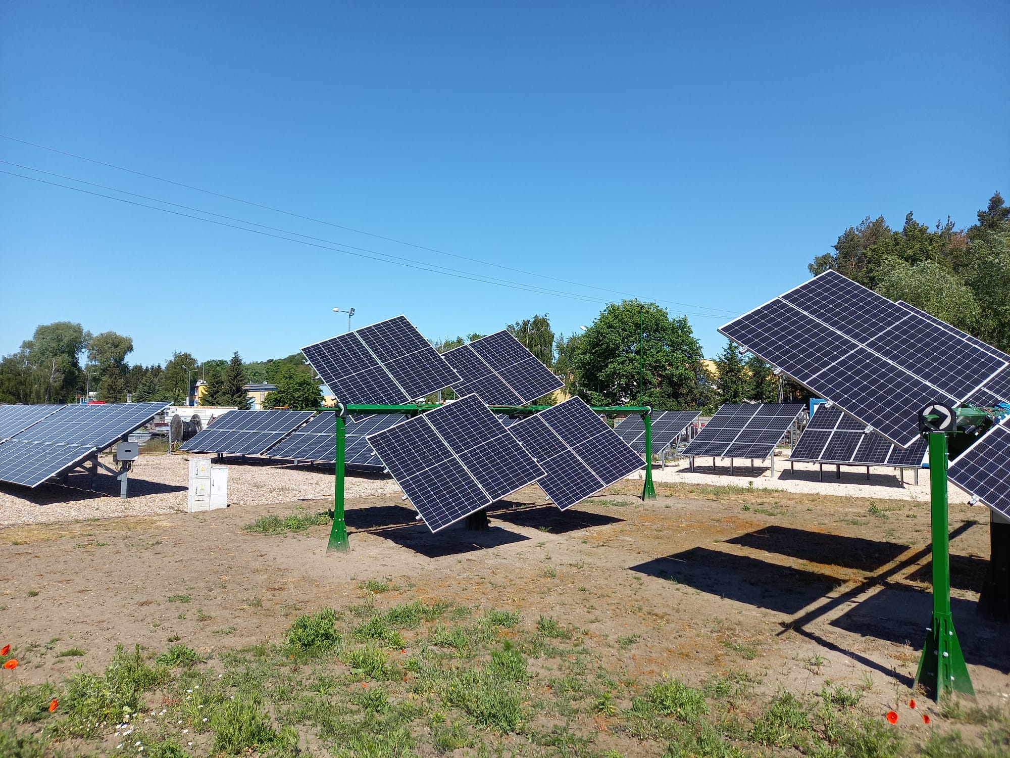
The photograph above is instructive: at that operating position, adjacent MODMEC collectors are not visibly shading one another, and the open support geometry does not cast a visible shadow across the module faces. That is valuable physical evidence about the photographed configuration. It is not a substitute for checking every relevant sun angle and tracker position through the year.
Latitude changes the geometry of the problem.
The same GCR does not represent the same operating compromise everywhere. At higher latitudes, winter solar elevation is lower, shadows are longer and seasonal variation in the solar path is greater. A spacing that performs well in Tucson may therefore produce a different shading pattern, tracking envelope and hourly profile in New York or Boston. Two-axis shading research explicitly identifies latitude, field layout, collector shape, tracker height and terrain as relevant variables.[5]
Tucson and San Diego also should not be treated as equivalent merely because both are far south of New York and Boston. Tucson typically offers a stronger direct-beam resource, while coastal San Diego can have more marine cloud and diffuse irradiance. New York and Boston combine lower winter sun paths with different cloud, temperature and snow conditions. Latitude changes solar geometry; local weather changes the resource available to that geometry.
Dual-axis comparisons require geometry-specific modeling.
Conventional fixed-tilt and single-axis models often infer shading from regular rows. Dual-axis systems add a moving collector surface, a movement envelope, a rotation point and more possible shadow relationships. Applying a generic tracker label or one GCR value is not enough.
A credible comparison needs the actual collector dimensions, pivot height, rotation limits, row and column spacing, terrain, collision clearance and control strategy. Otherwise the model can overstate both the feasible density and the energy yield.[5]
Annual MWh per acre are only the first layer.
Annual energy density answers an important question: how much electrical energy is produced from the selected acreage boundary over a year? But two systems with the same annual MWh per acre can produce very different amounts before 10:00, after 16:00 or during the site's highest-value hours.
For land-constrained projects, a stronger comparison can include annual MWh per gross acre, morning and late-afternoon MWh per acre, direct-to-load MWh per acre, curtailed MWh per acre, storage throughput per acre and time-weighted energy value per acre.
The economic denominator must also be consistent.
More usable energy from the same parcel can improve land productivity, but only if the additional structure, drives, controls, civil works, maintenance and financing do not consume the benefit. Siting constraints and community, environmental and land-use requirements also remain project-specific.[6]
The useful question is not “Which tracker makes the most energy?” It is “Which complete system produces the highest risk-adjusted value from the constrained site and connection?”
The MODMEC hypothesis.
MODMEC's design hypothesis is that independently controlled dual-axis collectors can combine a broad generation profile with a compact, accessible field layout. The open support geometry visible in the field installation is intended to limit structure-cast shading and preserve useful clearance around the modules.
The value of that approach should be tested at the project level—not inferred from annual tracking gain alone. The result may vary by latitude because the seasonal solar path and shadow geometry change, and by climate because the direct and diffuse components change.
TESTABLE SCENARIO
Hold the site constant. Then change the location.
Start with the same DC capacity, load profile, POI limit, battery and gross acreage in Los Angeles. Compare fixed tilt, single-axis and the MODMEC configuration using the same modeling boundary.
- Run a GCR and spacing sensitivity for each configuration.
- Measure annual, pre-10:00 and post-16:00 MWh per gross acre.
- Measure direct-to-load energy, curtailed energy and storage throughput per acre.
- Repeat the same design in Tucson and New York using site-specific weather files.
- Add San Diego and Boston when equivalent location inputs are available.
Differences between locations should not be attributed to latitude alone. The test changes both solar geometry and local weather resource; the model should report those effects separately wherever possible.
Open the MODMEC simulatorThe decision rule.
Treat land productivity as an hourly system outcome. Define the acreage boundary, model the real geometry, use site-specific weather, expose the shading and control assumptions, and compare energy when it can actually be used or sold.
Only then does “value per acre” become a decision metric rather than a marketing ratio.